We do a bit of business planning work here at Regional Strategic, Ltd. Our president, Mark Imerman, cut his teeth on business planning as a market development economist at the Iowa Department of Agriculture and Land Stewardship. It that role, he assisted farm operators and investors develop marketing facilities for alternative crops. It was a strategy pursued by the State of Iowa to reduce dependence on traditional row crops during the farm crisis.
In that role, he generally produced complete business plans:
Business description and objectives
Management qualifications
Personnel biographies and job descriptions
Sources of technical support
Market analysis
Competitive analysis
Pro forma financial projections
Investment and capital needs
At Regional Strategic, Ltd., however, we seldom get requests for the whole ball of wax. We primarily get contracts to do the market and competitive analyses. It is challenging and satisfying work. Every product, region, and delivery channel presents a different situation. All of these efforts are unique.
One thing we seldom see, anymore, is a full pro forma financial layout in small business development. This is true whether we are asked to help with small business planning or we are looking at plans done by others. Instead of detailed breakdowns of revenues, expenditures, and investment needs by month, we see rough annual estimates of total payrolls, start-up costs, production volume, and revenue.
This is unfortunate. The estimates might be well-informed and accurate, but the lack of detail is unfortunate, nonetheless. Annual estimates don’t match up revenues and expenditures as they occur. This is important, particularly in a small business startup. Without this, initial cash needs might be substantially underestimated simply because of mismatches between the accrual of expenditures and the realization of revenue. Annual estimates also hazard the risk of overlooking costs that might be incidental in and of themselves. These costs, in aggregate, can often be consequential. Missing them can result in material differences in overall estimates. There are often underestimation issues with startup costs, as well.
All of these factors increase the financial risk of business startup investors. They also increase uncertainty upon the part of potential lenders. This often results in elevated interest and insurance costs. In combination, these result in fewer small business startups in any given community. This reduces community income which reduces community tax revenues and impedes the improvement of community services. In short, they retard a community’s growth potential.
A five-year monthly pro forma financial layout encourages a business owner to walk through the first 60 months month-by-month. Properly set up, it will allow the investors and lenders to do what-if scenarios easily.
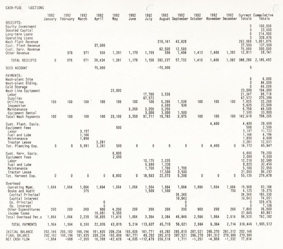
The table below is the fifth-year cash flow layout of one of Mark Imerman’s first business planning exercises. This particular plan specified financial requirements for a contract service provider engaged in planting, harvesting, packaging, and selling an alternative perishable food crop in Iowa. The spreadsheet analysis was set up with a single sheet of annual assumptions regarding acreage, service costs, output, waste, and revenues. Numbers in the cash-flow layouts were calculated from these assumptions. As a result, basic changes could be made concerning expected costs, acreages, yields, and sales prices, and those changes would automatically change the annual cash-flow layouts, which, in turn, would ripple through the annual operating and balance statements.
Pro forma financials are powerful tools. They result in better informed and prepared business owners, more confident investors and lenders, and increased potential for business growth within a community.
This was a relatively small investment project. It required a direct investment of about $130,000 and long-term loans of about $220,000 at the time. Given inflation, that is nearly equivalent to a total investment of $700,000 today. Long-term loans to accomplish this investment would likely have not been available in the absence of the pro forma analysis.
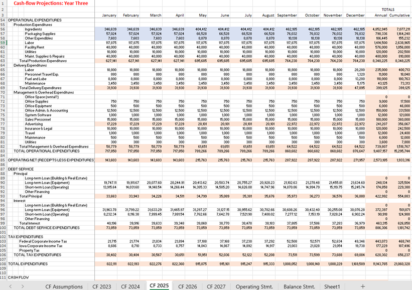
The second table shows a more recent example. It represents a potential frozen food manufacturer serving a limited geographic market in the upper Midwest. Figure Two shows the third-year expenditure portion of a five-year pro forma. Along the tabs at the bottom of the screen shot, you can see sheets for five years’ cash flows, balance sheets, and operating statements. There is also an assumptions sheet that drives cash-flow calculations. Cash flow calculations drive operating statements and balance sheets.
A set-up like this allows developers and investors to walk through alternative scenarios. You can see that production expenditures increase across the year. This reflects a scenario where output is still growing as the initial investment matures. Delivery expenses do not grow on the same schedule as production expenses. This reflects the lumpiness of delivery investments. All of these things become obvious when working through monthly pro forma cash flow projections. They are easily missed in annual lump sums.
Overall, the more recent operation is larger than that represented in the first table. The more recent table is part of the projections for a $5,000,000 investment. Generally, Regional Strategic, Ltd. works with business planning projects with investments between $500,000 and $15,000,000. It is a market segment that almost always benefits from a rigorous estimation of expenses and revenues.
The Iowa Legislature is currently working on a bill (SF 615) to impose work requirements on able bodied adult recipients of Medicaid. The bill passed the senate on Tuesday, March 27. It was passed with amendments by the house on Wednesday, March 28, and sent back to the senate. It will likely be passed and signed into law during the week of March 31, 2025.
On the face of it, it is kind of hard to figure out what this means. The governor apparently put forth the bill, but neither the governor’s office nor the departments of health & human services, public health, revenue, or management & budget provided any information to the Legislative Service Bureau on costs, savings, or fiscal implications of the bill.
Either they don’t know, don’t care to know, or don’t want anyone else to know the implications of SF 615. One can easily find estimates on the internet that 75 percent of Iowa adults on Medicaid already work, but it is hard to determine the potential exemption status of the other 25 percent.
To its credit, the Legislative Service Bureau did provide some important estimates to underpin the analysis presented here:
The bill will generate Medicaid savings of $3.1 million to the State of Iowa in the first year
The bill will generate savings of $17.5 million in the second and subsequent years
The funding percentage split between federal and state is 88.4 percent federal and 11.6 percent state
This means that when the state saves $3.1 million in the first year, the federal government will save $23.6 million, and when Iowa saves $17.5 million the second year, the federal government will save $133.4 million. Summing these up, during the first year while the State of Iowa is saving $3.1 million it will be cutting health care expenditures in the state by $26.7 million. During the second year the state will save $17.5 million by cutting statewide health care expenditures by $150.9 million.
So far, this has all been derived directly from the estimates made by the Legislative Service Bureau.
The United States Bureau of Economic Analysis (BEA) generates estimates of expenditures for each state. Assuming the healthcare expenditures eliminated by SF 615 are spread through the system on an equivalent basis to Iowa’s overall health expenditures, they can be run through an input-output model to see how they will affect the entire Iowa economy. The model was set up using coefficients available from the BEA.
Four scenarios were set up – two each for first year and for second year reductions in health care expenditures. In the first scenario for each year, health care expenditures were cut, and no other changes were made. In the second scenario for each year, it was assumed that the State of Iowa’s estimated savings were concurrently returned to taxpayers as household income (equivalent tax cut scenarios spread proportionately to income distributions).
Scenario One: First year health care expenditure cuts without equivalent tax reductions
State of Iowa savings – $3.1 million
Health care expenditure cuts – $26.7 million
Statewide payroll reductions – $17.3 million
Statewide jobs reduction – 307 jobs
Reduction in statewide returns to capital (profits, interest, rents, etc.) – $10.9 million
Job losses will fall predominantly in these sectors:
Health care – 189
Finance & real estate – 28
Professional, management, & administrative – 23
Wholesale & retail trade – 21
Additionally, a very rough estimate of state general revenue fund tax loss can be made by dividing state net tax deposits (Iowa Department of Revenue) by earnings by place of work (BEA) for Iowa. That calculation results in 8.75 cents in general fund tax deposits per dollar of payroll in the state.
This estimated tax loss would be $1.5 million. It would not include losses in non-general state income, such as the lottery or liquor, and it does not include local government receipts, but it would still amount to approximately half of the state’s anticipated savings from restricting access to Medicaid.
Scenario Two: First year health expenditure cuts with equivalent general tax reductions
State of Iowa savings – $0 (all savings are distributed in an equivalent tax cut)
Health care expenditure cuts – $26.7 million
Statewide payroll reductions – $16.4 million
Statewide jobs reduction – 287 jobs
Reduction in statewide returns to capital (profits, interest, rents, etc.) – $10.0 million
Estimated general revenue tax losses – $1.4 million
Job losses will fall predominantly in these sectors:
Health care – 185
Finance & real estate – 24
Professional, management, & administrative – 21
Wholesale & retail trade – 17
Scenario Three: Second year health expenditure cuts without equivalent tax reductions
State of Iowa savings – $17.5 million
Health care expenditure cuts – $150.9 million
Statewide payroll reductions – $97.7 million
Statewide jobs reduction – 1735 jobs
Reduction in statewide returns to capital (profits, interest, rents, etc.) – $61.5 million
Estimated general revenue tax losses – $8.5 million
Job losses will fall predominantly in these sectors:
Health care – 1068
Finance & real estate – 155
Professional, management, & administrative – 128
Wholesale & retail trade – 119
Manufacturing – 38
Scenario Four: Second year health expenditure cuts with equivalent general tax reductions
State of Iowa savings – $0 (all savings are distributed in an equivalent tax cut)
Health care expenditure cuts – $150.9 million
Statewide payroll reductions – $92.9 million
Statewide jobs reduction – 1620 jobs
Reduction in statewide returns to capital (profits, interest, rents, etc.) – $56.7 million
Estimated general revenue tax losses – $8.1 million
Job losses will fall predominantly in these sectors:
Health care – 1047
Finance & real estate – 134
Professional, management, & administrative – 121
Wholesale & retail trade – 95
Manufacturing – 33
Some thoughts
Regardless of the merits of imposing work requirements where the great majority are already working (recall that the governor and affected state departments declined to provide details regarding those merits), this is not simply a state budget reduction effort. It will significantly affect payrolls, employment, profits, and tax receipts across the state.
These effects are magnified by the fact that the federal government multiplies Iowa’s investment. For every dollar the state puts into these benefits the federal government contributes $7.62. That means that for every dollar the state saves with SF 615, the state forgoes $8.62 in economic activity that generates payrolls, employment, profits, and tax revenue. The state savings of $17.5 million per year will cost the state’s economy almost $151 million in expenditures (economic activity) per year.
The magnitude of these losses, particularly in the health care industry, will force providers to abandon billions of dollars worth of investments in facilities and infrastructure. These abandonments will not magically reappear if SF 615 is subsequently modified or repealed.
It should also be noted that, as expenditures fall, payrolls are cut, profits disappear, and jobs are axed it will be harder for Medicaid recipients to find the required jobs. This will remove more of them from Medicaid. This will save the state more money. For every dollar saved in this manner, another $8.62 in health care expenditures will be removed from the economy and the cycle of disruption to the state’s economy will continue to expand.
These are a costs that deserve more analysis than the governor or the statehouse has given.
We are doing some market analysis in Texas and surrounding states. One of the issues is to identify populations that might be potential purchasers of a particular offering. That is at least partially a function of income.
The graph below shows estimates of real per capita income trends within Texas household income quintiles.
For this graph, we didn’t work with any of the detailed categories. We stuck with total personal income.
Data came in a zip file with data for every state from 2012 to 2022. There were separate workbooks for every state. For every state there were separate worksheets for every year. Job one was to extract the data and combine all the years for Texas.
The downloaded data was not adjusted for inflation. We could easily see that some quintiles had seen income growth. With others, however, we could not immediately see if that was growth or if that was inflation. Step two was to download Consumer Price Index (CPI) data and adjust all of the years and quintile values to 2022-equivalent dollars. CPI data is available for download at https://www.bls.gov/cpi/data.htm. We used data for all urban consumers in the Southern region of the U.S. We used annual measurements that were not seasonally adjusted.
With inflation-adjusted data for quintiles of Texas households, we still could not see if individuals were gaining or losing ground. This is because every year the quintiles each give data for one-fifth of the households, but we have no idea of household or population growth.
We made a simple assumption that households averaged the same size across all five quintiles. That allowed us to take annual Texas population estimates divided by five as the number of people in each quintile. Dividing inflation-adjusted quintile incomes by population gave us the per capita income estimates shown in the graph. We utilized Texas population estimates from the BEA at https://www.bea.gov/data/by-place-states-territories, because data from the BEA is remarkably easy to locate, download, and use.
There are a few things about the data and the data manipulation that deserve note.
First, for every year the total income received by the top quintile was greater than the income received by the bottom four quintiles combined. This was not changed by any of the manipulations described above.
Second, the assumption that household sizes are the same across all quintiles was convenient and gave us the ability to normalize the data for population size but is probably not completely accurate. For any quintile where household sizes are larger than the overall average, the quintile’s per capita estimate would shift down. Conversely, for any quintile where households are smaller than the overall average, the quintile’s per capita estimate would shift up.
Our best guess is that the lower quintiles have larger households and that the higher quintiles have smaller households. This is consistent with the demographic arguments in the recent post, “The Coming Depopulation.” If so, the lines for the bottom quintiles would drop and the lines for the top quintiles would rise.
Third, the data estimates current realized income. That is pretty close to total income for the bottom quintiles. Households in the upper quintiles, however, are likely to have significant levels of unrealized unearned incomes in the form of appreciation or capital gains on investments. These streams are reported and show up in the data as they are realized. If they are realized in a constant steady stream over time, the data is probably an accurate reflection of reality. To the extent that unrealized income streams are growing over time, the data will underestimate them during any period.
This was an interesting exercise undertaken as part of a larger analysis of market potential in the Southern U.S. It is possible to replicate this for any state and to engage the data at a more specific level. While multistate regions can also be analyzed, they require additional manipulation because income ranges on household quintiles will be unique to every state. In all cases, a careful disclosure of assumptions made and the potential implications of those assumptions is required.
I am a recovering economist. I spent most of my adult life with production functions, growth models, economic impact studies, and such. Traditional economic practice and the concepts of progress it embodies assume things grow. Sure, there are recessions. There are depressions. There are areas of the world that stagnate and decline. Those, however, are aberrations. They are failures of individuals or small groups of people. They grow out of market failures that can be identified and cured. At least, that’s the theory…
While we studied the concept of scarcity when we learned price theory in introductory microeconomics the production functions in upper-level micro seldom have explicit limits. It is assumed that individual players are too small to affect total supply or demand, so individual players appear to have an unlimited supply of resources at their disposal. It is only a small conceptual jump for most of us – even those of us who are economists – to internalize the assumption that the resources of production are unlimited.
Input-output systems utilized in economic impact modelling explicitly assume unlimited linear production relationships. It is possible in the context of these models to define an economic event that will employ an additional 10,000 workers in areas having populations of less than 10,000. The model will dutifully crank out an impact to scale (for a quick look at some of the implications of this, see my blog post at Regional Strategic, Ltd.)
Beyond economic impact modeling, whenever we perform cost-benefit analysis looking forward, we discount future costs and benefits on the basis of some factor (generally an assumed future interest rate). The effect of this is that current benefits nearly always swamp future costs. Future costs approach zero the farther out we look because the discount rate reduces them at a geometric rate. In a world of limited resources, one might think that future costs should approach infinity as we run out of valuable stuff to consume, but that is not how we model the future. Our modeled perceptions are probably some distance from our grandchildren’s coming realities.
The Coming Depopulation
These ubiquitous assumptions of continuous growth are running headlong into the reality of worldwide population decline. This is not the Malthusian catastrophe or Paul Ehrlich’s population bomb. It is not due to famine or war ignited by overpopulation, poverty, and despair. The simple fact seems to be that as people around the world are getting better off they are having fewer children.
This reinforces theories of economic demography which suggest that in poor societies children are demanded as a form of insurance against illness, injury, and incapacity. Where infant and child mortality are high, this generates a substantial demand for more children as a hedge against both poverty and mortality. On the other side of the coin, in rich societies with low infant and child mortality and significant insurance infrastructures, the increased demand for children is channeled into quality rather than quantity. In this sense, children in rich societies are acquired much like luxury durable goods – why have a Chevrolet when you can have a Mercedes? Fewer children have greater opportunities to participate in elite sports or arts groups, get more prestigious educations, and, later in life, receive larger inheritances. This increases the status of their parents as an exclusive cadre of exceptional children is paraded about town.
This, to varying degrees, increasingly appears to be the situation around the world, at present. For individual families and children, it is a favorable development. Society wide, perhaps, not so much.
Worldwide population decline has not been experienced since the 14th century when the great famine and the bubonic plague savaged the known world in quick succession. That episode, however, generated substantially different demographic effects than we can expect from the current depopulation of choice.
The famine and the plague inevitably victimized weaker segments of the population – likely the elderly and the infirm – at greater rates than they affected the stronger. As population declined, the working-age population increased relative to other population segments. This increased the productive potential of the population that remained. As total population declined, it also bid up the wages of the working population that remained. Finally, because they inordinately victimized the elderly, the twin catastrophes accelerated intergenerational transfers of wealth.
As a result, the famine and the plague increased the productivity of the remaining population and redistributed wealth towards the working portion of the population. It is quite likely that the rapid population and wealth redistributions of the 14th century were substantial factors in the coming of the renaissance in the 15th and 16th centuries. In other words, increasing the proportion of the productive labor supply in the population and increasing the proportion of society’s resources available to that productive labor supply helped usher in two centuries of phenomenal economic innovation and growth.
The coming depopulation of choice will have very different ramifications. The coming depopulation will be the product of millions of decisions to have fewer children. That will mean fewer people entering the labor force. At the same time, increasing life expectancies will result in an increasing number of older people who have left the labor force. Unlike the 14th century situation in which the relative size of the working-age population increased and the relative size of the elderly population decreased, in the coming depopulation there will be an increasing proportion of elderly matched against a decreasing labor force.
Increasing the relative size of the elderly population can also be expected to decrease the resources available to the working-age population for two reasons. First, it will be necessary to commit an increasing share of output to a population that is no longer productive. Second, as people live longer, the intergenerational transfer of wealth slows. When people die at 50, inheritances accrue to people who are 30 and improve the lives of the dependent children of those beneficiaries. On the other hand, when people die at 80, the inheritances accrue to people who are 60 and will be held by those beneficiaries to support their coming unproductive years.
In the coming depopulation, we can expect the remaining population to become less productive because of the resulting age distribution and the reduction in resources that can and will be dedicated to support the productive portion of that population.
The Current Situation
In affluent countries, where life expectancies are high and premature death rates low, the replacement birth rate is approximately 2.1 children per adult female. This replaces two parents and accounts for pre-adult mortality. In less affluent countries, where pre-adult mortality rates are higher, the replacement rate must also be higher. In 2022, fertility rates in every region of the world except Africa, the Middle East, and Central and South Asia were below affluent-society replacement rates (2.1 children) and falling. Even the fertility rates in regions above the replacement level are falling. With the exception of Sub-Saharan Africa, fertility rates are below 3.0 for all of the above-replacement regions.
The population in China is already falling. East Asia as a whole has a fertility rate of only one-half the replacement level. The fertility rate in India is already below the replacement rate, as is true of all four of the world’s most populous countries (India, China, the United States, and Indonesia). While these trends are increasingly becoming the subjects of attention, they have been recognizable in every region of the world since at least the 1960s.
The United States is not experiencing depopulation. Fertility in the United States, at 1.6 births per female, is far below replacement levels, but strong immigration supports continued growth in the United States population. On the basis of current trends, the United States will continue to have an increasing population until about 2080, but current trends are largely dependent upon immigration.
As outlined in the previous section, the coming depopulation will be accompanied by significant aging in the population. Over the past 30 years, the proportion of the population over the age of 65 has increased by about 15 percentage points in East Asia, 10 percentage points in the European Union, and 5 percentage points in the United States. At varying rates, this trend is occurring in every region of the planet.
As the elderly live longer, working-age people move into the ranks of the elderly, and low birth rates fail to replenish the labor force, fewer and fewer productive people will be supporting larger and larger unproductive populations. In addition, as the elderly live longer, intergenerational transfers of wealth will slow and will become almost entirely transfer cycles within a multigenerational elderly population – continually concentrating resources within the ranks of the unproductive population.
The two demographic solutions to this are higher fertility and accelerating elder mortality. Neither of these appear to be on the horizon anywhere in the world.
Potential for Immigration and Replacement
In spite of sub-replacement fertility, the United States still experiences population growth due to strong levels of immigration. This immigration is driven by the need for labor force replacement in the United States coupled with a positive wage differential between the United States and the immigrants’ home countries.
These two factors are in place throughout the Western industrialized world. While Europe is increasingly concerned about immigration, Europe needs immigration to support its labor force. Hostility towards European Union immigration rules was a major instigator driving the Brexit movement, but Great Britain still needs to fill the labor gaps generated by an aging population with a declining labor force.
The wage differential between the United States and the undeveloped areas of the world (particularly Latin America) all but guarantees immigration, legal or illegal, into the United States. The same is true for Western Europe, particularly with respect to the Middle East and Africa. No nation has ever been able to stop economically driven immigration. In fact, dedicating significant resources in the attempt to stop such immigration will almost certainly exacerbate the internal labor force issues that are the major drivers of immigration in the first place. At best, nations can hope to shape the quality and quantity of their immigrant packages through carefully integrating national entrance and foreign policies.
A major issue with the labor force needs of the developed world is the skillset of immigrants from areas of the world with surplus populations. In an increasingly technical world, labor force needs will require immigrants with substantial skills. In contrast, it is estimated that 90 percent of young people in Sub-Saharan Africa and India, the two largest pools of remaining non declining population in the world, lack basic skills. To a lesser extent, this is also true of Latin America, the Middle East, and the rest of South Asia. These people are drawn to the labor shortages and wage differentials of the developed world, but they are not equipped to contribute at the levels required. The immigrant labor the developed world desperately needs is woefully educationally deficient.
What the Situation Requires
At its base, a solution to the problems that will accompany global depopulation and aging must revolve around increasing economic productivity. This is such an urgent need that the September 2024 issue of the International Monetary Fund’s Finance & Development publication is titled, “PRODUCTIVITY and how to revive it.” As smaller and smaller populations of productive people are left to support the needs of larger and larger unproductive aging populations, we will need to either generate increased levels of output from the productive population or succumb to decreasing standards of living for the population as a whole.
There are basically three means of increasing productivity:
Increase the availability of resources.
Increase the technical ability to transform those resources into goods and services that generate income and wealth.
Increase the skills of the population engaged in resource transformation.
The first of these offers, at best, limited potential. Having treated resource availability as infinite for over three centuries since the industrial revolution, the world’s available resources are becoming harder and harder to locate, develop, and acquire. In fact, the world is dedicating increasingly large shares of the second and third factors of increased productivity to the acquisition of the first. It is not a zero-sum game, but diminishing returns are certainly a reality.
The second requires investments in basic research that almost certainly will have to come from public initiatives. Private entities will willingly invest in the specialized research and development needed to bring marketable products into production. They will not, however, invest in the basic research and scientific progress that underpin their specialized research activities. Basic research results in knowledge available to any private entity. An individual corporation cannot engage in basic research because the successful results of that research do not accrue specifically to the corporation. The results might actually give competing corporations an edge in the marketplace.
Without public investment, basic research falters. Without basic research, productivity falters.
Unfortunately, in both North America and Western Europe, the cores of the world’s basic research infrastructure, levels of funding for basic research are falling. The public appetite for funding basic research through the expenditure of tax revenues has diminished. As a result, it will be very difficult to significantly increase the efficiency with which we transform resources into income and wealth as the world depopulates and ages. This does not augur well for the future.
In addition to funding, increasing basic research capabilities requires maintaining and improving the quality of students entering the various fields of basic research. This fits hand in hand with the third means of increasing productivity: increasing the skills of the population engaged in the transformation of resources.
Both the second and the third means of increasing economic productivity require continuous improvement in basic education. This should drive increasing commitments to and investments in education. As the working-age population diminishes, it is absolutely necessary that the skillset of the working-age population expands. This is immediately true in the developed world, where populations are aging rapidly, and working-age populations are shrinking rapidly. It is also necessary in the less developed world, which will inevitably be asked to replenish the shortfalls in developed nations’ productive workforces.
Unfortunately, public investments in education are also in decline in the United States and across Western Europe. The simple truth is that all three of the necessary components for increasing productivity and maintaining incomes in a depopulating and aging world are going in the wrong direction in the only areas of the world with the resources to improve them.
It gets worse. Even if the developed world invests in domestic education and research to improve productivity, it is almost certain that domestic productivity cannot be raised fast enough. The rapid declines in productive populations juxtaposed against the rising economic needs of an expanding elderly population will almost certainly outstrip even extraordinary productivity improvements. Additionally, the ability to raise the productivity of what are already the highest productivity populations in the world will be limited.
The simple fact of the matter is that maintaining income and wealth for the developed world will require augmenting the developed world’s labor force with imported labor, immigrants. In a world where most available immigrants lack the basic skillsets to be productive participants in a technical industrial and service economy, those skills will have to be improved before they immigrate.
This will require the developed world to invest in the educational advancement of less developed nations which can provide immigrants. This will have to be done by developed nations for two reasons. First, less developed nations simply cannot afford to upgrade their educational systems and human capital fast enough to address the immigration requirements of depopulation and aging in the developed world. Second, educating potential immigrants from the less developed world, like basic research discussed above, will not generate value that the host countries can directly capture. In fact, the very premise, here, is that the people educated will migrate from their less developed home countries to the developed world.
If they desire to maintain their income levels in the face of depopulation and aging, developed countries will have to invest heavily in improving both their own education and human capital development systems and education and human capital development in the less developed world. In addition to maintaining their own income levels, this will have an impact on improving income levels for the world as a whole.
Not all newly educated youth in the less developed world will migrate out. That will improve the productive human capacity of their home countries. It can also be expected that a substantial proportion of the immigrants to developed countries will remit earnings to their home countries. This may not sound familiar, but it has parallels to the situation discussed above concerning the twin catastrophes of the 14th century. By increasing the productivity of the workforce in less developed countries and providing additional capital to that workforce (through both external investments in education and emigrant remittances), we might create conditions for at least some of those less developed countries to take off.
Conclusion
The coming world depopulation appears to be set in stone. Over half of the people in the world live in countries where fertility rates fall below replacement rates. All four of the most populous nations in the world (India, China, the United States, and Indonesia) fall within this group. Only three broad regions on Earth have fertility rates above the replacement level: Africa, the Middle East, and South Asia. Fertility rates are falling in every nation on Earth, even in countries where fertility remains above replacement levels.
Depopulation due to declining fertility rates inevitably means populations will age significantly. Rising proportions of elderly people juxtaposed against declining productive populations will result in declining incomes unless rates of economic productivity increase substantially.
The central component to increasing economic productivity is education. Maintaining income levels in the coming depopulation will require an immediate commitment to increase investments in education. This will be necessary but not sufficient in the developed world. It is also imperative that the developed world make an immediate commitment to increase educational investments in less developed countries. This is necessary because the developed world will be dependent upon technically proficient immigrants to augment its labor force as its populations shrink and age.
We are doing some work on farm and farmer value streams here at Regional Strategic, Ltd. The pilot work is using Iowa, but the intent is to take what is found and expand the work across the Upper Midwest.
One of the first major questions regards farmland valuation and appreciation. The graph below shows a simple relationship that leads to a number of complex questions. The graph shows cumulative inflation-adjusted value streams for ag land appreciation (from Iowa State University’s Farmland Value Survey), direct government payments (from the Bureau of Economic Analysis), and farm income net of government payments (derived from the Bureau of Economic Analysis) per acre of farmland (from the Census of Agriculture).
The period runs from 1993 to 2022. The scenario assumes that an acre of land is purchased in 1992 and the purchaser initiates production in 1993. The three lines show accumulations of income and land appreciation over a 30-year period. The endpoint is set as the last year in which complete stable information was available from the Bureau of Economic Analysis.
The first thing that jumps out is that accumulated land value appreciation outruns operating income and direct government payments. Accumulated land appreciation separates from the other two streams in 2002. In addition, Operating income breaks out above direct government payments in 2007.
Over the thirty years, the three inflation-adjusted value streams generated an average of $458 per year. Averages for each of the components were
Of this average value stream, only 38 percent came from income, and nearly a third of this income was in the form of direct government payments. Operating income accounted for only a little over 26 percent of the value stream generated by an average acre of Iowa agricultural land.
Average farm earnings net of government payments (operating income) was only sufficient to pay a 4.72 percent return on the 1992 purchase price of $2,559. Operating income plus direct government payments were only sufficient to pay 6.86 percent return to purchase price. This is all barely enough to cover interest or carrying cost on the investment.
Given these low production returns, what makes land price appreciation average 11.5 percent per year?
What caused land appreciation rates to break away from operating income and direct government payments in 2002?
What caused operating income to break away from direct government payments in 2007?
A portion of these relationships might simply be the result of the period being observed, but the size and consistency of the breaks suggest there is something more. There appears to be a confidence in the value of Iowa farmland that overrides observed farmland productivity. Why is that?
Is it due to indirect subsidies?
Is it due to the conviction that subsidies and relief will always maintain farm income?
Is it because of a belief that the removal or reduction of farm subsidies, both direct and indirect, will inordinately affect other production areas and concentrate production and value in Iowa?
We honestly don’t know the answers to these questions. That is the point of the inquiry. More will come as we noodle this out.
Interested in Learning More About Regional Strategic, Ltd.? Send Us a Message