Over the past several weeks, I have heard multiple farmers say that, while prices are really bad right now, they are still a buck or two higher than when Biden was president. I didn’t believe them for a minute, but, at the same time, I don’t believe they were lying to me.
Our minds all work to make sense out of the thousands of bits of information we encounter each day. We unconsciously build a story that makes consistent sense of our current experiences and our deeply held beliefs. As a result, we all firmly believe some things that are somewhat less than true. We truly believe them because they are consistent with our understanding of ourselves. If you care to delve into this phenomenon, I suggest picking up a copy of Daniel Kahneman’s Thinking, Fast and Slow.
Anyway, while these gentlemen were not lying, they were passing on untruths. It is likely that presenting facts in response will have no effect upon what they believe, but facts are available, and I am going to run through a few of them here.
This is about more than prices for a bushel of corn or soybeans. A buck or two on Iowa’s 2.7 billion bushels of corn and 600 million bushels of soybeans is 3.3 to 6.6 billion dollars, or 2-3 percent of Iowa’s personal income. The gain or loss of a buck or two on a bushel of corn or soybeans is important to the state’s economy as a whole.
As farmers spend or don’t spend this level of money, revenues surge or dry up for local car dealers, dance instructors, restaurants, and grocers. This determines whether kids wear new shoes to school – farm kids and non-farm kids alike. Voting on the basis of falsely held beliefs regarding commodity prices affects the entire community – not just the farmer. The discussion that follows attempts to put some values on these impacts for Iowa.
USDA Market Year Prices
We start with market year average prices from the United States Department of Agriculture (USDA). Market years run from September 1 of the harvest year to August 31 of the following year. They coincide with the expected period during which a producer markets the current harvest.
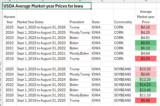
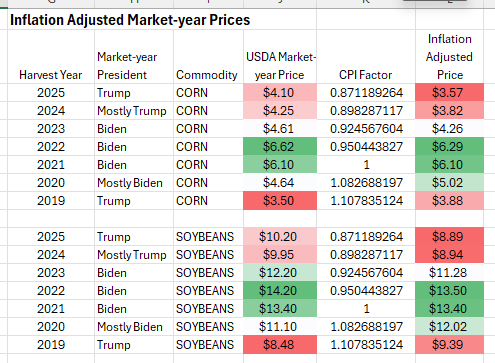
The table below shows USDA average market year prices for corn and soybeans from the 2019 harvest year to the 2025 harvest year in Iowa. The table includes market year dates for reference. It also indicates who was president during the market year. The lists of market year prices for both corn and soybeans were given a color-gradient scale with Excel. Red indicates the lowest prices. Green indicates the highest prices. All of the red occurs in Trump presidencies. All of the green occurs during the Biden presidency.
The price range for corn over the seven market years is from $3.50 per bushel to $6.62 per bushel. The range for soybeans is from $8.48 per bushel to $14.20 per bushel.
Adjusting for Inflation, Adding Production Levels, and Generating a Weighted Average Inflation Adjusted Price for the Period
The discussion above is sufficient, in and of itself, to address the price comments we have heard from farmers. These differences, however, have significant effects on Iowa’s non-farm economy. To show that, we need to demonstrate the effect that these price swings have on the overall income – farm and non-farm.
Inflation Adjustment
We start by adjusting the market year prices for inflation. At a per-bushel level over seven years this is not hugely important. If we are to look at overall income, however, we have to multiply per-bushel prices by total production. A ten-cent price difference multiplied times 2.5 billion bushels of corn is 250 million dollars. To avoid this variance, we used the Consumer Price Index (CPI) for all Midwestern urban consumers to standardize dollar values across the period.
We made the assumption that USDA market year prices were representative of prices at the midpoint of the market year. We then averaged CPI indices for February and March of the years 2020 to 2026 to coincide with the midpoints of the 2019 to 2025 market years. We then used those averages to standardize our USDA market year prices on the dollar value at the midpoint of 2021 market year (February-March of 2022). The year was chosen because it matches the current set-up of the economic impact model we will be using below. It has no effect on results.
Inflation adjusted prices are shown in the table below. Once again, the prices were placed on a color-gradient scale.
Adding Production, Realized Income, and a Weighted Average Price
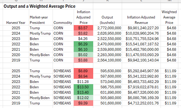
To get to total incomes related to the price variations we see, we add bushel output for both corn and soybeans through the period. Output numbers are from the USDA and represent the harvest years coinciding with the market year prices utilized above.
To generate income or realized revenue, we simply multiplied inflation adjusted prices times output levels to get inflation adjusted revenue for each crop year.
Then we divided the sum of inflation adjusted revenue by the sum of output across the seven years to generate a weighted average price for the overall period. Our weighted average price for corn is $4.68 per bushel. For soybeans, $11.09 per bushel. Both weighted average prices are denominated in dollar values current at February-March 2022.
The Difference Between Realized Revenue and Baseline Revenue
We used realized income in the table above to generate a weighted average price for both corn and soybeans across the seven-year period. The weighted average price can be used as a baseline of sorts to reflect expectations. We can multiply the weighted average price times annual production values to get a baseline revenue value or expected revenue relative to any year’s production volume.
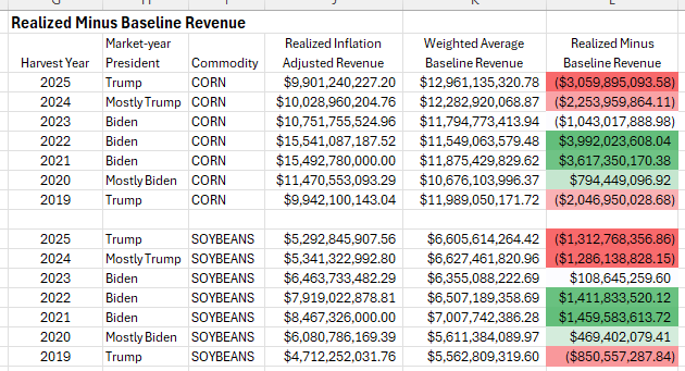
We can then subtract our calculated value of baseline revenue from our calculate value of actual inflation adjusted revenue to generate a measure of realized farm revenue divergence.
We have done that in the table below. We have used Excel to place a color gradient on the series. Red represents a large negative divergence (expectations are much higher than realizations). Green represents large positive divergence (expectations are much lower than realizations).
For corn, our divergences of realized to expected revenues ran from a deficit of over $3 billion to a surplus of nearly $4 billion – a spread of nearly $7 billion.
For soybeans, our divergences of realized to expected revenues ran from a deficit of $1.3 billion to a surplus of nearly $1.5 billion – a spread of nearly $2.8 billion.
These variations all represent farm income. At this point, we have made no assumptions or estimates on how these farm income fluctuations will affect the surrounding non-farm economy. They will have an effect, however. When farm incomes are flush, farmers spend extra money on new vehicles, recreation, goods, and services. When farm incomes are short, farmers economize on these expenditures.
Non-farm Impacts of Farm Revenue Variations
Because we are working only with final price variations and production is fixed, we can look at this variation in farm revenue as variations in farm family income. By the time commodity prices are established, all farm production activities and expenses have been realized. The economic impact of production is fixed. The economic impact of these income variations are entirely due to changes in the expenditures of farm families in the economy around them.
To get at this, we first combined the corn and soybean variations for every year (the far-right column of numbers in the table above). Then we ran these summed variations in farm income for every year through an economic impact model generated with Regional Input-Output Multiplier System coefficients from the U.S. Bureau of Economic Analysis (BEA). We then used the CPI to adjust the dollar values to reflect dollar values at the midpoint of the 2025 market year (February-March 2026) to bring the values into line with current price experience.
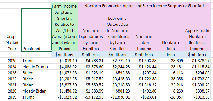
The results of this are shown in the table below. The first column of numbers (under the green-shaded heading) is the sum of the corn and soybean income variations from the table above after adjusting to February-March 2026 dollar values. This is the effect that revenue surpluses or deficits from our weighted average price directly affect farm families in Iowa. In the 2025 line, this figure reflects a shortfall of slightly over $5 billion in Iowa farm income relative to expectations based on our weighted average prices for corn and soybeans.
The next five columns (under the plum-shaded headings) show the off-farm impact of these farm income variations. The first of these columns shows changes in non-farm expenditures by farm families. In the 2025 row, for example, we see that a farm income shortfall of just over $5 billion is expected to result in a nearly $4.8 billion reduction in farm family expenditures. This is money that is not received by businesses like auto dealers, grocers, dance studios, and restaurants around Iowa.
Of this $4.8 billion that Iowa businesses do not receive from farm families, nearly $2.8 billion is value that would have been created within the Iowa economy – “Value Added” in the language of economists. The remaining $2 billion would have consisted of goods and services imported from outside of Iowa.
The $2.8 billion in lost Iowa economic activbity would be split nearly evenly between labor income ($1.39 billion that would have supported over 28,000 jobs) and business income ($1.38 billion worth of business earnings, interests, rents, and a very small sliver of indirect business taxes).
You can run across any of the crop-market year lines and build a similar story. The column with the green-shaded heading represents the direct effect of expected price shortfalls on farm income. The columns with the plum-shaded headings shows how reduced farm income translates into reduced off-farm expenditures, payrolls, jobs, and business income.
Conclusion
This all started with a few farmers remarking that farm prices, while bad, are a couple of dollars higher than they were under President Biden. Even though it is easy to demonstrate that they are wrong, these farmers are sincere in their beliefs in this regard.
As a talking point, a couple of dollars on a bushel of corn or soybeans passes most of us without generating an awareness of billions of dollars in lost economic activity. This is unfortunate.
When we can promote simple erroneous statements as political talking points and ignore the fact that those erroneous statements mask billion-dollar swings in personal income and economic activity, we are encouraging people to vote in ways that are in direct opposition to their own self interests and the interests of their neighbors.
Nothing is more detrimental to faith in government than false political narratives that are demonstrably harmful to the very people they are targeted at.